Reread Classics/Translation: Facebook Ad Sorting Model: LR-GBDT
In an Internet industry that is constantly iterating and updating technology, there is a need to keep learning enthusiastic. The lesson of the front car, the teacher of the future, learn the valuable experience of the former, can take fewer detours, less to dig their own "pit". This is a paper published by Facebook in 14 years in which the classic (and now slightly old-fashioned) GBDT-LR algorithm is proposed. The so-called warm and new in re-reading this paper reflected in the most vivid, the first reading of the student era to pick up the algorithm framework on a taste of the end, after work and then read and found a lot of content closely related to the daily work: experimental design, feature system construction, online learning, sample sampling and so on. This highly engineering paper is worth reading carefully, the technology will expire, but the rigorous engineering thought is always quality. Share my translation of the paper below, if there are any leaks, please point out.
Long text warning!This article contains 16,261 characters.
Summary.
The primary purpose of an online advertising platform is to engage advertisers in bidding and paying for predictable behaviors, such as clicking on certain types of ads. It goes without saying that the Click Prediction module is the most important part of most online ads. Facebook not only has a billion daily users, but also more than a million active advertisers, predicting click-to-click is a challenging machine learning task. In this paper, an algorithm model combining decision tree and LR is proposed, which is more than 3% more effective than using both algorithms alone, which is a performance improvement that has a significant impact on the whole system. At the same time, this paper also explores how some basic parameters affect the predictive performance of the system.There is no doubt that the top priority is to have the right characteristics: the characteristics that capture the user's historical information and advertising advantage characteristics。 Once you have the right features and the right model (i.e., the decision tree plus LR just mentioned), the other elements play the role of a companion (even if a small increase is huge on a large scale for the population, it means that the lift is difficult). Choosing the best way to keep data freshness, planning learning rates and data sampling are all side roles that are not obvious to model improvements.It is far less important than adding strong features or choosing the right model。
1. Introduction
Digital advertising is a multi-billion dollar market, and that number is growing dramatically every year. In most online advertising platforms, ad distribution is dynamic and often tailored to the user interests that are tapped for feedback. Machine learning plays an extremely central role in calculating users' click expectations for candidate ads and accelerates the efficiency of the online advertising market in this way.
Google, Yahoo and Microsoft have all conducted research in computing advertising and are interested in finding relevant information. The efficiency of online advertising auctions depends on the accuracy and validation of click predictions. Click prediction systems need to be robust and adaptable, as well as the ability to learn large amounts of data.The main purpose of this article is to share insights into experimenting with real-world data while keeping an eye on robustness and adaptability。
In search advertising programs supported by major Internet companies, a candidate ad set that uses user-entered qury term retrieval and has an explicit or implicit matching relationship (the retrieval process can also be called a recall, or as part of a recall). In a Facebook scene, ads aren't associated with query, they're relatedDistinguish between target groups and point-of-interest positioningIt's all about. As a result, the number of ads that can be shown to users in this scenario is much larger than the number of search ads.
Every time a user visits Facebook, an ad request is triggered, and in order to handle the large number of ad candidate sets in each request, you first need to build a series of cascade classifiers that are increasingly computing costs. In this article, the discussion focuses on the last part of the cascading classifier, which is the click prediction model that gives predictions (click probability) for the final candidate set. Next, start with an overview of the experimental design in the second chapter. In the third chapter, different linear classifiers based on statistical probability are evaluated, and a variety of online learning algorithms are introduced. While discussing linear classifiers, the effects of feature transformation and data freshness on classifiers are studied. Inspired by lessons learned in practice, particularly around data freshness and online learning, Facebook engineers have come up with a model structure that incorporates the online learning layer while designing several fairly concise and robust models. The fourth chapter describes in detail the key components of the online learning layer, the online joiner, which is the basic component of the experimental part and is mainly used to produce real-time training data streams.
At the end of the paper, a variety of methods to balance memory and computational efficiency in processing mass training data are discussed. In Chapter 5, you share a variety of practical tips for preventing potential memory problems when dealing with large-scale applications. Then in Chapter 6, we discuss in depth how to balance the amount of training data with the accuracy of the model.
2. Experimental settings
To ensure the rigour and controllability of the experiment, a training dataset was constructed using a week in the fourth quarter of 2013. At the same time, in order to ensure the consistency of training data and test data under different conditions, offline training data similar to online observations are prepared, and training and test sets are divided from these offline data to simulate the flow of online training and prediction. All experiments in this article use the same training/test data.
Evaluation metrics: Since we should be most concerned about the impact of various factors on the machine model, it is more reasonable to use the model predictions directly than the real profits and revenues. In this article, the main useStandard entropy(Normalized Entropy, NE)和Calibration rate(Calibration) as the main evaluation indicator.
Standard entropy, more accurately, standard cross-entropy, equal to the average log loss per exposure divided by the log loss corresponding to all exposures predicted by the model for the potential CTR (background click through rate). Background CTR is an average of the empirical CTR (empirical CTR) for the entire training dataset, and perhaps it is more appropriate to call it standardized log loss, and the smaller the value, the better the model predicts. The main reason for standardization is that when the background CTR is closer to the log loss of 0 or 1, the better the log loss, divided by its entropy in order to make the standard entropy insensitive to it. Suppose a training sample is thereNsamples, indicates whether to click, Represents the probability of clicks predicted by the model. Represents the average of empirical CTR, and the calculation of standard entropy is shown below.
Formula (1):
NE is essentially used to calculate relative information gain (Relative Information Gain, RIG), and the relationship between the two is RIG = 1 - NE。
Calibration rate is the ratio of estimated average CTR to empirical CTR, in other words, the ratio of expected clicks to real clicks. It is a very important indicator and is an essential step in estimating CTR validation as a good online bidding and auction platform. Closer to 1 represents the more accurate the model's prediction. Since the specific data are not published, this indicator is only described in the experiment. It's worth noting that the AUC (Area-Under-ROC) is also a good indicator of evaluation. But in the real world, we hopeForecasts are more accurate, not just to optimize the ranking, to avoid potentially poor or excessive delivery。 The standard entropy evaluates the predicted good or bad, while implicitly responding to the calibration rate. For example, if a model gives twice the predicted value of the real value, then we need to multiply it by 0.5 for calibration, and the corresponding standard entropy will increase, but the AAUC will remain the same.
3. Predict the structure of the model
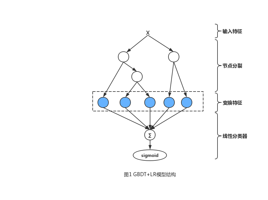
As shown in Figure 1, this section focuses on a hybrid model:Series gradient lift tree (GBDT) and sparse linear classifier (LR)。 In 3.1, we demonstrated that the decision tree can be effective for inputFeature transformations greatly improve the accuracy of linear classifiers。 3.2 Mainly shows how fresher training data can lead to more accurate predictions, which is why we use online learning methods to train linear classifiers. Then, in 3.3, a series of online learning variables are compared for two different probability linear models (LR and Bayes).
In studying e-learning scenarios, we evaluated the application of random gradient drop algorithms (Stochastic Gradient Descent, SGD) to sparse linear classifiers. After a feature change, each exposed ad can be used as a vector to represent, which Represents No i unit vectors, Is. n Category input features. The same is used during the training phase Mark whether the ad has been clicked. For an exposure ad with a tag , the predicted score of the model can be used
Formula (2):
to indicate, Represents the feature weight vector.
According to the traditional Bayesian online learning scheme for probit regression, BOPR, conditional probability and a priori probability can be expressed
which A distribution function that represents a standard positive distribution, represents a density function. BOPR achieves online training through expectation propagation with moment matching, which results in acquisition The average and variance of the approximate post-test distribution of . The reasoning process of BOPR is computation and then maps it to by reason decomposition the approximate Gaussian approximation. As a result, the update algorithm only needs to consider that the probability is not 0 the average and variance of . The following is a simple inference process, interested can be carefully studied.
Formula (3):
Formula (4):
Formula (5):
Appears above And. (Note and distinction) is a penalty function, defined with And. indicates that the reasoning process is similar in And. use SGD. We liken the BOPR analogy to an like-for-like function
Over here. That's the LR we're familiar with. The reasoning of LR is mainly based on the use of the number of like-for-like guidance, using the SGD algorithm to update the parameters according to the step of the gradient. As shown in formula (6). Formula (6):
which represents a gradient of a non-zero element, for step length. LR algorithm is very simple, gradient calculation process uses a lot of guidance techniques, here is no longer more detailed, there is a need to consult the relevant information. It's worth noting that both BOPR and SGD-base are stream learners that need to fit training data step by step.
3.1 Decision tree feature transformation
There are two simple ways to characterize the input features, which can improve the accuracy of linear classifiers. First, the nonlinear transformation techniques that are commonly used for continuous features areDiscrete(box, bin) becomes a categorical feature. Linear classifiers can efficiently learn these segmented features. It's important to let the model learn useful bin boundaries, and there are a lot of information maximization methods to do that.
The second simple but effective feature transformation isThe combination of features。 For class features, the most brutal combination is the use of Descartes, which means that all the original features are combined. Obviously, not all combinations are valid, but it's bad that those that don't work aren't easy to get rid of. If the entered feature is a continuous feature, you can also use feature combinations, such as the kd tree for joint binning.
In our study, we found that gradient lift trees can transform features very effectively and lightly through the discrete and combined methods just mentioned. Each tree is treated as a category feature, with the number of samples falling on the leaf node as the feature value, and eventually the feature is encoded using one-hot. For example, the ascending tree in Figure 1 has two sub-trees, which contain three and two leaf nodes, respectively. If the sample falls on the second and first leaf nodes in two trees, the one-hot encoded feature can be represented by a vector of 0, 1, 0, 1,0, which represents whether the first three elements in the vector represent whether the sample falls on the leaf node corresponding to the first tree. The gradient lift tree used in this article is derived from the classicGradient Boosting Machine algorithm and adds L2 normals (now generally used XGBoost or LightGBM). In each round of iterative training, a new tree is generated to model the residuals of the previous tree. You can put itThe gradient lift tree feature transformation is understood as a supervised feature code, which transforms the original feature vector into a 0/1 vector, and the path from the root node to the leaf node represents the selection rule for the non-leaf node feature. The transformed vector is placed into a linear model to learn the weights of these rules。 Gradient lift trees typically train models in batches.
We experimented to verify the effect of decision tree transformation features as inputs on linear models, and compared two LR models in the experiment, the difference between the two models is whether to add these transformation features. At the same time, the experiment also compared the model using gradient lift tree prediction alone, the specific results are shown in Table 1.
| Model. | NE |
|---|---|
| GBDT+LR | 96.58% |
| LR | 99.43% |
| GBDT | 100% (control) |
As can be seen from Table 1, the LR model using conversion characteristics has decreased by 3.4% compared to the NE indicator of a single GBDT model, which is a stunning improvement in the real world. For reference, a set of typical feature projects can only bring about a decline in the NE index of dozens of percentage points, most of the characteristics of engineering experiments only a few percentage points. Interestingly, using LR and tree models alone has acquaintance accuracy (LR is slightly higher), but when combined, there is a qualitative leap.
3.2 Data freshness
Click prediction systems often exist in dynamic environments, and the distribution of data that needs to be processed changes over time. Next, the effect of real-time training data on prediction effect is mainly studied. To do this, we train the model based on a certain data and use it to predict data for six consecutive days. In terms of the model, two models, GBDT and GBDT-LR, are selected, and the NE indicator is calculated as shown in Figure 2.
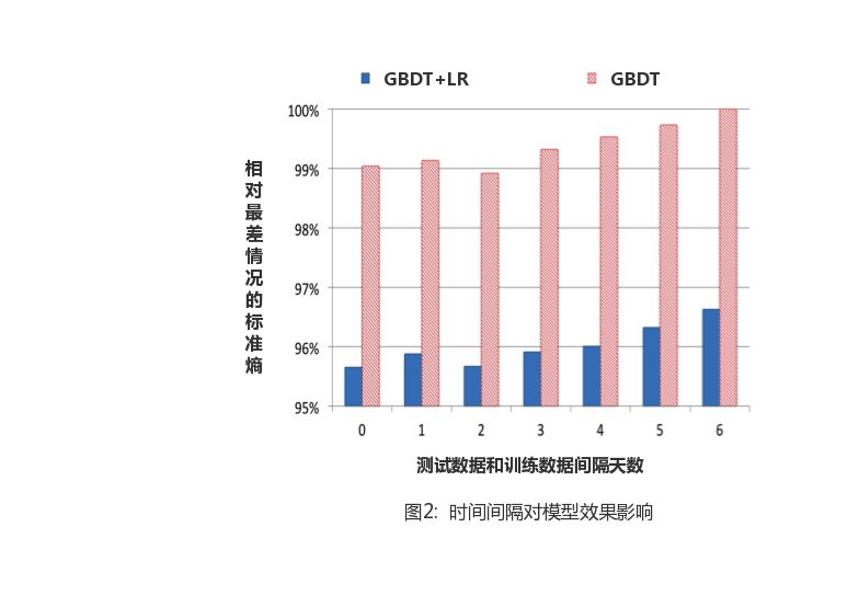
It is obvious from the figure thatAs the interval between test and training sets becomes longer, the model becomes less effective。 From the performance of the two models, the weekly update model compared to the day-to-day update model, the NE indicator loss of about 1%, which also showsIt is necessary to update the model at the day level。 One possible scenario would be to build a repetitive daily task to train the model, preferably in batches. In practice, the update cycle of the gradient lift tree is determined by many factors, including the number of training samples, the number of trees, the number of leaf nodes, CPU, memory, and so on. Training a boosting model of hundreds of trees for hundreds of millions of samples can take more than a day on a single-core CPU. In a real-world production environment, the training process can be compressed to several hours through distributed processing such as multi-core machines. In the next chapter, we'll talk about another viable alternative, that isDecision trees are still trained in days or days, while linear classifiers (LRs) can take advantage of some of the features of online learning for near real-time training。
3.3 Online linear classifier
In order to maximize the freshness of the data, one option is to train the linear classifier directly using real-time click information for exposure ads. Later chapter four will detail how to generate real-time training data, the main content of which is to evaluate several algorithms commonly used to update learning rates in LR online learning. Then, find out where the best results compare with the BOPR model. According to Formula (6), we explored the following learning rate update methods:
Adaptive learning rate (Per-ability learning rate): For features i In the first t The learning rate of the round iteration
which is an adjustable parameter (the idea comes with a citation).
Single-weight square root learning rate (Per-weight square root rate learning):
which represented until the first t Wheel-to-round characteristics i All training sample data.
Single-weight learning rate (Per-weight learning rate):
Global learning rate:
Constant learning rate:
The first three scenarios set different learning rates for each feature, and the last two scenarios share the same learning rate for all features. With grid search, the best parameters for each scenario are shown in Table 2. The lower limit of the learning rate is set at 0.00001 during training, and the LR model is trained and tested using the above schemes on the same data set, and the final experimental results are shown in Figure 3.
| The update method | Parameters. |
|---|---|
| Adaptive learning rate | |
| Single-weight square root learning rate | |
| Single-weight learning rate | |
| Global learning rate | |
| Constant learning rate |
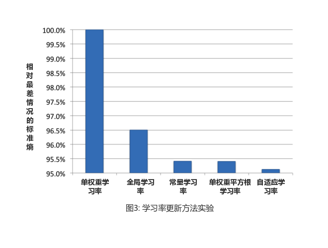
Interestingly, the average in the UPDATE formula (3) in the BOPR model is very similar to the adaptive learning rate in the SGD-based LR model update. The effective learning rate in BOPR is based on a specific dimension and depends on the post-test variance of that dimension and the deviation predicted by the previous model. As shown in Table 3, we also compared the predictive performance of the LR model and the BOPR model using adaptive learning rates. In the experiment, both models were trained with the same data set and then evaluated for accuracy in predicting the next day. As expected, due to the similarity of the update process, the performance of the two models in evaluating indicators is similar.
| Model. | NE |
|---|---|
| LR | 100% (control) |
| BOPR | 99.82% |
Compared to BOPR,The advantage of LR is that the model size is only half that of the former, mainly because LR only needs to calculate the weight of the feature, not the average and variance. Given the online deployment, the smaller the model can optimize cache locality to speed up cache hits. For the calculated cost of prediction, the LR model only needs to take the internal product of the calculated feature vector and the weight vector, while the BOPR model only needs to co-accumulate the feature vector with the variance vector and the average vector, respectively.
The advantage of BOPR ratio over LR is that, as the Bayes formula is applied, itProvides a complete predictive distribution of click probabilities。 This can be used to calculate the percentile of the predicted distribution, which is useful for exploring and developing learning scenarios.
4. Online data join
The previous chapters mentioned that fresh data can improve predictive accuracy and proposed a simple model framework for online training. This chapter focuses on an experimental system that is primarily used to generate real-time training data required for online learning. Because its key role is in the online environmentJoin tags (click) and training input (ad exposure), we call this system an "online joiner" (Online Joiner)。 Similar structures are also used in streaming learning, such as Google's advertising system. The online joiner outputs real-time training data streams to Scribe, Facebook's open source log collection system.
A positive sample can be well defined by clicking, but there is no "no click" button available to the user. That's why,Ads that do not generate clicks are generally used as a negative sample, but the length of time an ad stays (exposure duration) is controlled. It is important to note that you need to be very careful about adjusting the window size of the negative sample length of stay。 Using too long a window can result in delayed push of real-time training data and increase memory overhead due to exposed ads waiting for click signals. The problem with setting up windows that are too short is that click information is lost because the corresponding ad exposure is quickly refreshed resulting in a false mark as a negative sample. This negative effect interferes with click coverage, which is the proportion of clicks in all exposures. Therefore, the online joiner system must be weighedTime-thy-time and click-to-over。
Incomplete click overlay meansThere is bias in the real-time training set: The predicted experience CTR is lower than the real CTR. That's because some exposure samples marked as clickless should be click samples when the time window is long enough. However, we found that in a real-world environment, this bias can easily be reduced to a few percentage points by setting a reasonable window size, and that these small biases can be calculated and corrected. Online data joins are designed to complete ad exposure and clicksStream-to-stream data consolidation, the most important component of which is the request ID. Every time a user triggers a content refresh action on Facebook, a request ID is generated. Figure 4 briefly describes the logic of linking from online to online learning.
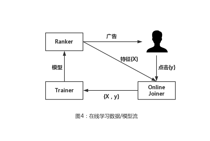
When a user visits Facebook, the first stream is generated, which then triggers Ranker's sort request for the ad candidate set. The ad is then pushed back to the user, and each exposure ad and associated feature is added to the exposure stream. If a user clicks on an ad, the click message is also added to the clickstream. In order to achieve stream-to-stream data joins, the system uses a first-in-first-out policyHash queue(HashQueue) is also used as a cache windowHash table.for quick and random access to exposure labels. A typical hash queue has three operations for key-value pairs: join, out, and find. For example, for an element (advertisement), we need to add it to the head of the team and add a key-value pair to the hash table to mark it and its position in the hash queue. Only if all join windows expire will the exposed ads be pushed to the training stream. If you don't click on the association, the exposed ad will be marked as a negative sample.
In this implementation system, Trainer periodically releases new models to Ranker by constantly learning about the training data stream. The result is a tight closed loop for machine learning models that capture and learn feature distributions in a short period of time, as well as performance monitoring and real-time tuning of models. When we experimented with training data generation systems in real time, we realizedThe importance of establishing protection mechanismsThe role of the protection mechanism is to deal with the abnormal phenomenon of potential corrosion of the whole online learning system. For example, when a clickstream cannot be refreshed because of an error in the underlying data facility, the online joiner produces training data that can only learn a small (or even zero) predicted value, followed by an online classifier that incorrectly estimates a very low click-through rate. Because ad exposure depends on the model's predictions, low predictions can lead the system to reduce the number of ads exposed. Exception detection is useful in this case. For example, when the distribution of online real-time training data changes dramatically, the system can automatically cut off the connection between online Trainer and Online joiner.
5. Optimize memory and latency
5.1 Increase the number of trees
In the gradient lift tree model, the more trees there are, the longer it takes to predict. In this section, we study the effect of the number of trees on model accuracy.
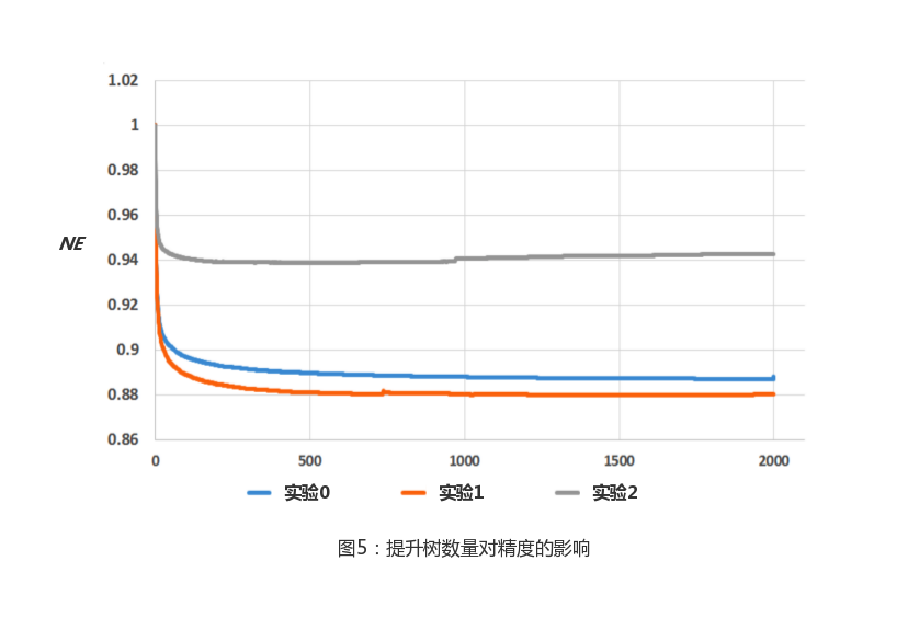
As shown in Figure 5, we trained a GDBT model of 1-2000 trees using data from the same day to predict the next day's data, controlling each tree with fewer than 12 leaf nodes. As in a series of previous experiments, standard entropy is used as an evaluation function. As the number of trees increases, the NE continues to decline. However, the benefits of increasing trees are declining, with the last 1000 trees bringing about less than 0.1% change in the indicator, and even the model numbered 2 has an accuracy fallback after 1000 trees. The reason is that model 2 uses four times less data training than other models, resulting in overfitted phenomena.
5.2 Raise the importance of tree characteristics
During model building,The number of featuresis an important factor in balancing predictive accuracy with computational performance. In order to better understand the impact of the number of features, we first need to define the importance of each feature. We use statistics Boosting Feature Importance The importance of calculating features, the idea of which is to calculate the cumulative loss reduction for each feature contribution. Each node in the tree picks an optimal feature as the basis for the split, maximizing the decrease in square error. Because the same feature is available in multiple trees, the statistic is equal to the amount of error drop for a particular feature in all trees. In general, a small amount of features contains most of the explanatory information, and most of the remaining features contribute very little (Marginal benefits)。 By drawing an example diagram of the number of features and their importance (Figure 6), we confirm the relevant laws.
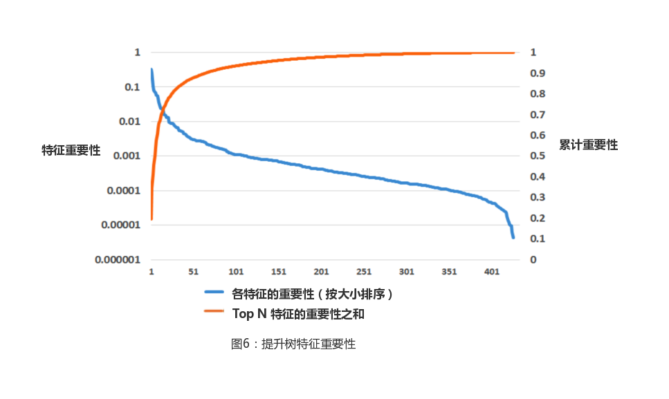
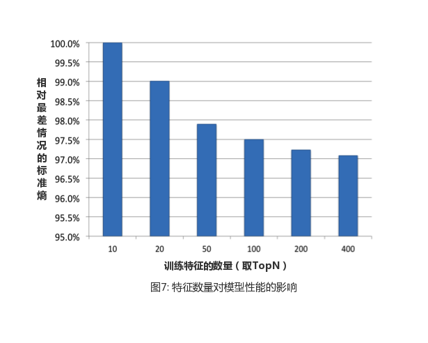
The results from the graph found that the top 10 features contributed nearly half of the "importance", compared with the last 300 features contributed less than 1%. Based on this finding, we conducted further experiments to explore how the number of features affects performance by retaining only the top 10, 20, 50 and other features for model training. The results of the experiment are shown in Figure 7, and the increase in the number of features results in a decrease in the benefits of the evaluation indicators.
In the next chapter, this article explores the usefulness of historical and contextual features. Details of these characteristics cannot be disclosed due to data sensitivity and company policy. Context features mainly include time, date, and so on, historical characteristics can be the historical click statistics of ads and so on.
5.3 Historical features
Features used in the lift tree model can be grouped into two categories:Contextual features and historical features。 The value of context characteristics is reflected in the unique environment that describes the current exposure ad, such as the device used by the user or the page currently viewed. Instead, historical features depict the historical (behavioral) information of a user or ad, such as an ad's click-through rate in the past week or the average click-through rate in a user's history. In this chapter, we focus on the performance of these two types of features in the system. First, we examine the importance of these two types of characteristics. To do this, we sort all features by important, and then calculate the historical features before k the proportion of features, the results of which are shown in Figure 8.
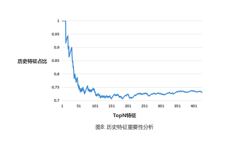
As can be seen from the results,Historical features provide more useful information than contextual features, the importance of the top 10 are historical characteristics. Although historical features account for about 75% of all features in the entire data set, there are only two contextual features in the top 20. To better understand the differences between the two types of features, we trained only two models using one class, and we also trained models that contain all the features. The result of the comparison is shown in Table 4.
| The type of feature | NE |
|---|---|
| All features | 95.65% |
| Historical characteristics | 96.32% |
| The context feature | 100% (control) |
Based on the evaluation indicators in the table, we can confirm once again that historical features in general play a more important role. In the absence of historical features, the accuracy of model loss is 4.5%. In contrast, removing contextual features results in a loss of less than 1%. It should be noted that contextual characteristics are in responseCold start(cold start) plays a very important role in the problem. For new users and new ads, it's essential to get a reasonable estimate of click-through rate context characteristics.
Next, verify the sensitivity of these two features to data freshness by evaluating the performance of models trained separately with historical or contextual features over a continuous period of time.
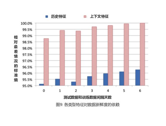
As shown in Figure 9, we find that models that utilize contextual features rely more on data freshness than historical features. This is in line with our intuition, because historical features describe the long-term behavior of the user and are more stable than contextual characteristics.
6. Processing of large-scale training data
Facebook's one-day ad exposure data contains a huge sample of values that can reach hundreds of millions of dollars, even if a small amount of valid data is not easily disclosed because of confidentiality. One of the common ways to accelerate model training is to reduce the number of training samples. This chapter focuses on two methods of undersampling:Uniform subsampling and negative down sampling。 For different sampling methods, the gradient lift tree model consisting of 600 trees is trained and the corresponding evaluation indicators are compared.
6.1 Even undersampling
Because.Even undersampling is easy to achieve, so it is the most common method of processing training sets, and the resulting model can act unaligned on the extracted training data and the unexered test data. In this section, we evaluate the sampling rate for approximate exponential growth, which is .0001, 0.01, 0.1, 0.5, 1. Based on the same basic data set, samples are obtained using each sampling rate to train the lift tree. The performance on the evaluation indicators is shown in Figure 10.
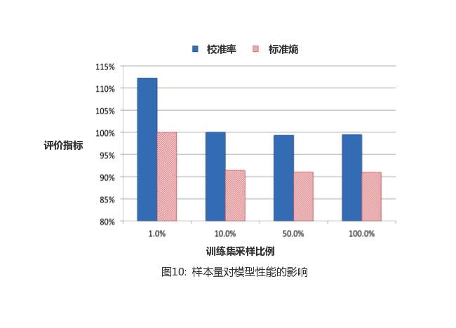
Consistent with our intuition, the more data you have, the better your performance. Not only that, but the increase in benefits from increased sampling rates is decreasing. Compared to the total data, the use of 10% of the data on the evaluation indicator loss of only about 1%.
6.2 Negative downsampling
Many scholars are rightLabel imbalanceIn-depth research has been carried out, and it has been proved that such problems have a very important impact on model performance. In this section, we will investigate the effect of using negative-drop sampling to deal with label imbalances (negative-drop sampling is to maintain a positive sample size and only undersampling negative samples). As a rule of law, we tried different negative drop sample rates to take samples for experiments, and the sample rate changes to .1, 0.01, 0.001, 0.0001. The final results of the experiment are shown in Figure 11.
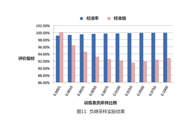
From the results, the take-out size of the negative drop sample rate has a great impact on the performance of the model, with the best performance value of 0.025.
6.3 Model calibration
It's mentioned aboveNegative downsampling speeds up the training process and improves model performanceNote that if the model uses downsampling, you need to calibrate the predicted values for the downsampling space. For example, assuming an average CTR of 0.1% before sampling, if we use a negative sample of 0.01, the model predicts CTR to be approximately 10% (100 times). In this case, we need to use a formula
Pulls the real-time stream prediction back into the 0.1% range, in the formula And. Represents the predicted value of the downsampling space and the negative sample rate, respectively.
Summary
In the above content, the actual experience in dealing with Facebook's real advertising data has been given. These valuable experiences underpin our design of a hybrid model structure that works well in the direction of click prediction.
Data freshness matters。 At least a retraining of the heavens is necessary. The paper is a step closer, discusses a variety of online learning programs, and also shares the system that generates real-time training data. The feature transformation of the gradient lift tree is obvious to the linear probability classifier。 From this point of view, a hybrid model structure combining lifting tree and sparse linear classifier is designed. Best way to learn online: UseAdaptive learning rate of LR。 Its performance is basically the same as THATR's, the model size is only half that of the latter, and it performs better than the LR model using other learning rate scenarios.
In addition, we describe techniques for dealing with memory and latency issues when developing large-scale machine learning applications.
It describes howWeigh model accuracy against the number of lift trees。 Choosing as few trees as possible can be very helpful in controlling memory and optimizing computing. Gradient lift trees can be easily carried out by calculating feature importanceFeature selection。 Helps us reduce the number of features without un as much impact on predictive performance. We analyzed the impact of using historical and contextual features on the model. For ad and users with a history,Historical features perform much better than contextual features。
Finally, we discuss various sample-downing scenarios, among whichNegative downsamplingis a simple and effective uniform method.
The translator of this article
Zhao Qun graduated from Harbin University of Technology's Intelligent Computing Research Center in January 2019 and joined shell language intelligence and search department after graduation, mainly engaged in search sorting optimization.
You may also want to read it
One mirror in the end: the principles of FM and the practice of shell search
Go to "Discovery" - "Take a look" browse "Friends are watching"